Setting up CSV files in Excel

Accelerus Icon
 

Although data may be added manually in Accelerus, it is not designed specifically for large amounts of data entry, but for adding of Accelerus-specific data, such as assessment items, plus the occasional new student, changing enrolments when a student moves classes, and so on.

It is well worth getting to know Microsoft Excel, as it can be used to:

Make the manipulation of data in the CSV files prior to importing easier, eg the data that has been extracted from your school's timetable may be missing some fields or their exact format is not correct.
Set up data from scratch, where it is not available from another source in electronic form at all.
Make bulk changes to records, eg where you want to change all of your subject codes.


minusFormat of data changes in Excel

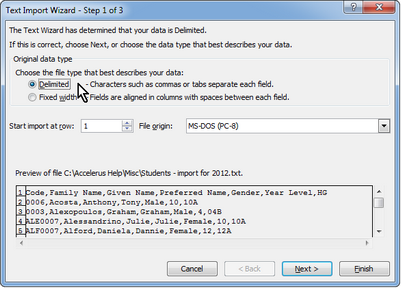
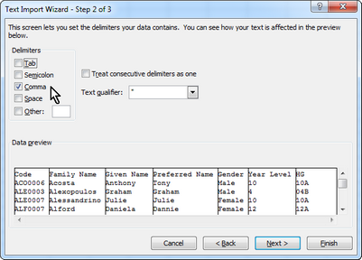
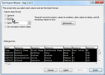
When a CSV file is opened in Excel, the format of all of the columns therein is automatically set to General. This format automatically converts what it thinks are numbers to numbers, anything that looks like a date, to a date, etc.

Therefore, if you have leading zeros on your codes, they will will be dropped off when you open the file. For example, student code 091111 will automatically become 91111.

Some of the problems with fields becoming dates occur with codes and subject levels. For example, code APR04 become 4 April, and a subject level of 8-10, ie it covers levels 8 to 10, becomes 8 October.

In order to combat these problems, there are two slightly different set of steps you can take, depending on whether you open the file from within Excel or double click it and launch Excel at the same time.

Create the file as a .txt file or even change the extension of the file to .txt.
Run Excel and then open the .txt file via the Open option in Excel.
In the first of three Wizard windows that will appear, make sure the Delimited option button is selected and then click Next.

CSV ExcelWizard1

In the second Wizard window:
®Remove the tick from the Tab delimiter box.
®Tick the Comma checkbox.
®Click Next.

CSV ExcelWizard2

In the last of the three windows:
®Check the Text column data format option.
®Highlight all of the columns appearing in the Data preview section.
®Click Finish.

CSV ExcelWizard3

OR

From Windows Explorer right click the file and select Open with Excel.

The file will open with each row being comma separated, but all in the one cell.

Select all of the data in the file.
In the Data ribbon click the Text to Columns icon.

CSV ExcelTextToColumns

The same Wizard windows as described above will come up and you should follow the same steps in this case also.
Make the changes you require in Excel.
Save the file as a CSV file.


Warning

If you need to open the CSV file again to make further changes, you must follow the same set of steps. Otherwise, the data will be changed back again.

Alternatively, if only minor changes are required, open the CSV file in a text editor such as Notepad.


minusSaving as a CSV file and not an XLS

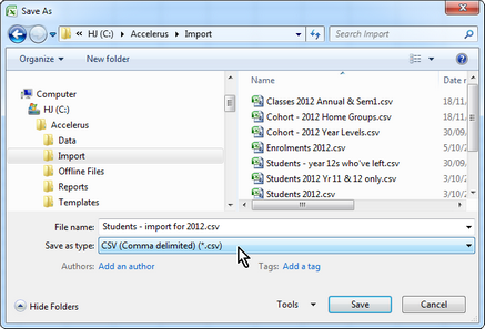
When you have finished editing a file in Excel that was not a .csv file to begin with, eg an .xls or .txt file, you must ensure that you select Save As and select CSV in the Save as type field in the Excel Save As window, as shown here.

CSV ExcelSaveAs

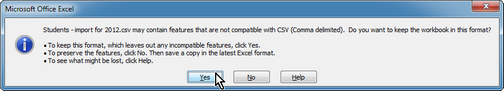
However, whenever you close a file you have been working on in Excel, having already saved it as a .csv file, make sure you follow these steps:

Click Yes when presented with the following message, which will vary a little, depending on the version of Excel you are using.

You must ensure that your file remains as a .csv file and not an Excel .xls file. Yes, is confirming you do want to keep the .csv format and not save it as a .xls file.

CSV ExcelSaveMsg

On closing the file in Excel, click No to the further message asking if you want to save the changes to the file - you already saved it as a .csv file in the previous step.

CSV ExcelNoChangesMsg

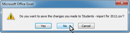
If you do not follow these steps, you will be presented with the Save As window again, and Excel will keep trying to save the file as a .xls file.


Lightbulb

Just remember, Yes to the first message, No to the second.


minusUsing Excel formulas to change data

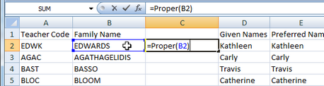
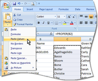
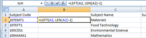
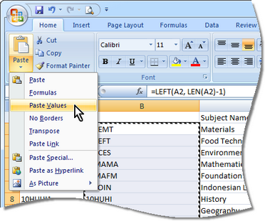
Often the data extracted from other sources may not have the exact format required to be imported into Accelerus. Or, it may be that you want to change some of the current data in Accelerus, eg remove or add a suffix to codes.

This is where Excel is extremely useful, as functions may be used to quickly change your data. Two typical examples of the use of Excel are outlined here:


Often student or teacher family names are in upper case and you may want them to be in proper case.

In Excel, insert a new column beside the field that you want to change to proper case, eg the family name
In the cell beside the first name, type in the formula shown below, substituting B2 with the appropriate cell reference for the name you are changing.

CSV ExcelProperFunction

Fill this formula down to all other rows in the file.
Copy the whole column.
Go to the Paste menu and select the Paste Values option.

CSV ExcelProperPasteValues

Delete the original upper case column, and make sure the new column has the correct column heading.
Check any names that may have capitals within them, such as McNabb, as you will need to change these manually. Names with spaces, hyphens or apostrophes will convert to proper case correctly.


Your subjects may come out of the timetable package with a 1 or 2 suffix – 07ENG1, 10CHE1, etc - but as you are using semester academic cycles in Accelerus, these are not required.

Create a new column in the .csv file, in Excel, beside the column containing the original subject codes.
In the cell beside the first code, type in the formula shown below, substituting A2 with the appropriate cell reference for the code you are changing.

CSV ExcelRemoveSuffix

Fill this formula down to all other rows in the file.
Copy the whole column.
Go to the Paste menu and select the Paste Values option.

CSV ExcelRemoveSuffixPaste

Delete the original subject code column, and make sure the new column has the correct column heading.


Lightbulb

If you have the other situation where you want to add a suffix or prefix to a set of codes, you may follow the same sets of steps as shown above but use the concatenate function, represented by the & character in the following formulae:

=B1 & "1"

OR

="1" & B1

Of course, enter whatever text you require as the suffix or prefix in the quotation marks, and replace the B1 with the appropriate cell reference.

You may also use concatenate to join together data from two or more columns.